One might think the analysis of a fluorescence decay is easy. In the end, it’s just standard curve analysis. However, the art is to precisely describe the fluorescence decay down to the shot-noise of the experiment. When doing so, a number experimental aspects have to be considered for the analysis: the instrumental response function, IRF, the differential non-linearity of the device, DNL, pile-up effects, etc.
The quality of the experiment limits the conclusions one can draw, and a poorly controlled experiment may never be analyzed down to the experimental shot noise. In this post, I will give recommendations on recording fluorescence decays of high quality, discuss fundamental limitations, and provide practical help for the analysis of fluorescence decays, which you would typically only get being part of a scientific research group dedicated towards fluorescence.
Instrument response function
IRF stands for instrument response function. In time-resolved fluorescence measurements the IRF is the temporal response of the fluorescence spectrometer to a delta-pulse. If a δ-pulse excites the sample the recorded fluorescence intensity decay solely depends on the meaured sample. Such “ideal” decay is illustrated below in the subfigure A. If the sample is excited by a broad pulse. The fluorescence intensity decay is a super position of multiple”ideal” decays, each has an intensity which is proportional to the intensity of the excitation pulse.
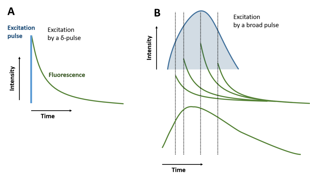
In practice, the excitation pulse width, the temporal dispersion of the fluorescence light in the instrument, and the detector contribute to the temporal response of the instrument, which has to be considered when analysing fluorescence intensity decays.